[机器学习]Linear Regression模型和优化方法

线性回归在机器学习任务中非常常见且，模型相对简洁易实施，值得仔细学习。

Linear Regression模型的基本任务

Linear Regression模型的基本预测方程:

\[\tag{1} \hat{y} = {w_1}{x_1} + {w_2}{x_2}+ ... + {w_n}{x_n}\]

用矩阵的形式表达为：

\[\tag{2} h_{w}(X) = {w}^T \cdot X\]

使用常见的MSE损失函数：

\[\tag{3} L(w) = MSE(X,h_{w}(X)) = \frac{1}{m} \sum_{i=1}^{m}(w^T \cdot X^{(i)} - y^{(i)})^2\]

则Linear Regression模型的优化目标是找到使损失最小的参数 $\hat{w}$。为解决线性回归问题，经典的机器学习算法（优化器）主要是正则方程（最小二乘法）和梯度法，其中最小二乘法在统计、微积分、线性代数、概率论等系统都有解释方法，梯度法则从基本的梯度下降法衍生出更实用的批量梯度下降、随机梯度下降和小批量梯度下降等经典算法。线性回归模型常见的是多项式回归，而对于实际问题中的非线性输出，传统线性模型无法做到因此引出逻辑回归，使用sigmoid等映射函数将输出映射到非线性空间去，除去映射函数其他步骤同传统线性模型并无区别。逻辑回归在多分类问题上的推广可使用Softmax回归，计算样本在多个类上的分数后，将得到最大概率的类别作为输出。

Normal Equation

Normal Equation(正规方程)十分简洁，对于上面给定的描述，其形式表示为

\[\tag{4} \hat{w} = (X^T \cdot X)^{-1} \cdot X^T \cdot y\]

正规方程是最小二乘解的矩阵形式。

实际上 X^TX 不可逆的情况非常少就算 X^TX 真的是不可逆也无妨，可以对原始数据进行特征筛选或者是正则化即可。

Normal Equation的推导和理解

从方程的角度看，方程（2）在现实中大部分情况是不可解的，所以进一步退而求其近似解 $\hat{w}$。

\[\hat{w} = arg\ min_w L(w)= arg\ min_w {||y-Xw||}^2\]

尝试展开L(w)有

\[L(w) = {||y-Xw||}^2 \newline = {(y-Xw)}^T(y-Xw) \newline = y^Ty-(Xw)^Ty-y^TXw+(Xw)^T(Xw) \newline = y^Ty - 2w^TX^Ty + w^TX^TXw\]

其中 $X^Tw^Ty$ 和 $y^TXw$ 得到的结果都是 1x1 的标量，对于标量 $a$， $a^T = a$，因此 $w^TX^Ty = (w^TX^Ty)^T = y^TXw$。

为最小化L(w)令其w的导数等于0有

\[\frac{ \partial L(w) }{ \partial w} = \frac{\partial ({y^Ty - 2w^TX^Ty + w^TX^TXw})} {\partial w}\]

其中

\[\tag{a} \frac{\partial (y^Ty)}{\partial w} = 0\] \[\tag{b} \frac{\partial (-2w^TX^Ty)}{\partial w} = -2X^Ty\] \[\tag{c} \frac{\partial (w^TX^TXw)}{\partial w} = 2X^TXw\]

由(a)、(b)、(c)可得

\[\frac{ \partial L(w) }{ \partial w} = -2X^Ty + 2X^TXw\]

令其等于0，可得

\[\hat{w} =(X^TX)^{-1}X^Ty\]

此处要求X矩阵是满秩矩阵。

矩阵求导可查询wiki，另附参考文档：matrix_rules.pdf

梯度方法

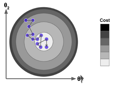
梯度方法是机器学习中最常见的优化方法之一，从微积分的角度看对多元函数的参数求偏导，把求得的各个参数的偏导组成的向量就是该多元函数在各个参数上的梯度。在几何意义上，梯度的指向的方向是增长最快的方向，因此朝着梯度相反的方向可以快速找到最小值从而达到优化目的。

梯度方法相关的几个重要因素：

步长：也即学习速率（learning rate），步长决定了每次梯度下降时参数变更的幅度。步长过打容易过冲无法找到最优点，步长过小结果更精确但训练将非常缓慢，
特征：输入部分的相关特征选取可以优化计算速度，特征工程方面的内容后面再作学习（先挖坑）。另外在预处理输入是对特征归一化处理可以加快梯度优化速度。
损失函数：一般使用MSE(L2损失)。因为他是凸函数，可以保证计算的是全局损失而不用担心可能算出一个局部损失(梯度下降不一定能够找到全局的最优解，有可能是一个局部最优解。如果损失函数是凸函数，梯度下降法得到的解就一定是全局最优解，凸优化的坑以后慢慢填)。相对于MAE（L1损失），MSE的鲁棒性更差（对异常点敏感）。

批量梯度下降 (Batch Gradient Descent)

批量梯度下降法是梯度下降法的最基本形式，其特点是每个参数每次迭代都在所有训练数据上的计算梯度（当前参数在损失函数上的偏导）:

\[\frac{ \partial L(w) }{ \partial w_j} = \frac{2}{m} \sum_{i=1}^{m}(w^T \cdot x^{(i)} - y^{(i)})x_j^{(i)}\]

矩阵形式为：

\[\nabla_{w} L(w) = \begin{pmatrix} \frac{ \partial L(w) }{ \partial w_0}\\ \frac{ \partial L(w) }{ \partial w_1}\\ ...\\ \frac{ \partial L(w) }{ \partial w_n} \end{pmatrix} =\frac{2}{m} X^T \cdot (X \cdot w - y)\]

Hands-On Machine Learning with Scikit-Learn and TensorFlow (Equation 4-6. Gradient vector of the cost function)
Notice that this formula involves calculations over the full training set X, at each Gradient Descent step! This is why the algorithm is called Batch Gradient Descent: it uses the whole batch of training data at every step. As a result it is terribly slow on very large training sets (but we will see much faster Gradient Descent algorithms shortly). However, Gradient Descent scales well with the number of features; training a Linear Regression model when there are hundreds of thousands of features is much faster using Gradient Descent than using the Normal Equation.

参数更新方法：

\[w^{j+1} = w^j - \eta \nabla_{w^j} L(w)\]

随机梯度下降 (Stochastic Gradient Descent)

批量梯度下降法对步长的取值比较敏感，过大则精度不够，过小则收敛太慢，此外由于批量梯度下降法需要对整个训练集计算梯度，当数据较大时计算过程较慢。随机梯度下降方法则是将随机抽样概念引入基本梯度下降算法，采取动态步长和训练部分随机样本的一种策略，目的是优化精度且兼顾收敛速度。

Hands-On Machine Learning with Scikit-Learn and TensorFlow (Page 117, Stochastic Gradient Descent)
Stochastic Gradient Descent just picks a random instance in the training set at every step and computes the gradients based only on that single instance. Obviously this makes the algorithm much faster since it has very little data to manipulate at every iteration. It also makes it possible to train on huge training sets, since only one instance needs to be in memory at each iteration (SGD can be implemented as an out-of-core algorithm.
On the other hand, due to its stochastic (i.e., random) nature, this algorithm is much less regular than Batch Gradient Descent: instead of gently decreasing until it reaches the minimum, the cost function will bounce up and down, decreasing only on average. Over time it will end up very close to the minimum, but once it gets there it will continue to bounce around, never settling down (see Figure 4-9). So once the algorithm stops, the final parameter values are good, but not optimal.

因为抽样的随机性SGD不能保证稳定地找到最优点，只能说是相对最优点，常见的解决办法是使用模拟退火算法（simulated annealing），开始设置一个较大的学习率，然后根据收敛程度逐步减小学习率，具体的学习率由学习率调度算法（learning schedule）决定。另一方面这种随机性可以使得SGD跳出局部最优点（Local Minima），因此在找全局最优点上SGD是比BGD更好的方法。

小批量梯度下降

不同于批量梯度下降法（每次使用整个训练集）和随机梯度下降法（每次使用一个抽样样本集），小批量梯度下降使用多个小批量随机样本（mini-batch）进行梯度迭代计算。Mini-bach GD在计算上对硬件更为友好（特别是GPU上）。简单来说Mini-batch GD速度比BSD快，比SGD慢；精度比BSD低，比SGD高。

\[w_i = w_i - \eta \sum\limits_{j=t}^{t+x-1}(h_w(x_0^{(j)}, x_1^{(j)}, ...x_n^{(j)}) - y_j)x_i^{(j)}\]

算法流程：

选择n个训练样本（n<总训练集样本数）
计算每个样本上的梯度
对n个样本的梯度加权平均求和，作为这一次mini-batch下降梯度
重复训练步骤，直到收敛

梯度法调优

算法步长
初始化
归一化
特征选取

梯度下降特点:

选择合适的学习速率α
通过不断的迭代，找到θ0 ... θn, 使得J(θ)值最小

正规方程特点:

不需要选择学习速率α，不需要n轮迭代
只需要一个公式计算即可

多项式回归（Polynomial Regression）

当数据更加复杂时一元的直线模型可能不那么好用了，很容易联想到可以将数据在多元方程上拟合。多项式拟合的做法是，将感兴趣的 feature 幂运算作为新的 feature 加入训到练集。

  
import numpy as np
from sklearn.preprocessing import PolynomialFeatures
from sklearn.linear_model import LinearRegression
%matplotlib inline
import matplotlib.pyplot as plt

m = 200
x = 6*np.random.rand(m,1)-3
y = 0.5*x**2 + x + 2 + np.random.rand(m,1)
print("%d,%d"%(len(x),len(y)))

plt.scatter(x,y)

poly_features = PolynomialFeatures(degree=2, include_bias=False)
x_poly = poly_features.fit_transform(x)
x_poly[0]
# array([-0.89981979,  0.80967565])

lin_reg = LinearRegression()
lin_reg.fit(x_poly, y)
lin_reg.intercept_, lin_reg.coef_
# (array([2.50385144]), array([[0.99925638, 0.49855815]]))

多项式回归和学习曲线（Learning Curves）

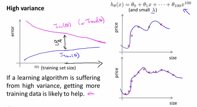
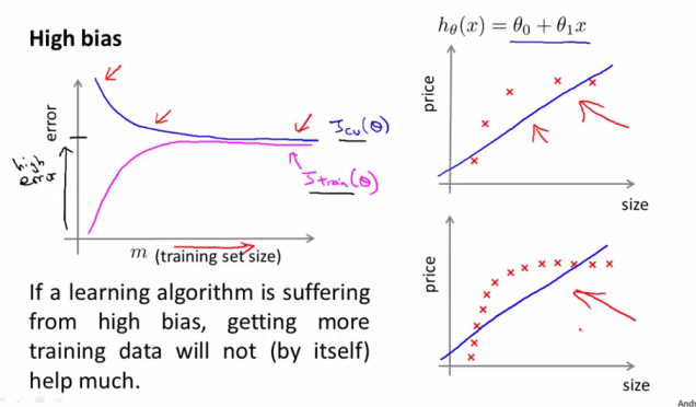
多项式回归中PolynomialFeatures的超参数degree对模型影响较大，选择的维度过小会出现欠拟合（高偏差），维度过大则不可避免的过拟合（高方差），衡量一个模型的拟合过于简单还是过于复杂一般使用交叉验证方法，另外一个方法就是看学习曲线（Learning Curves）图。

学习曲线的绘制方法是在多个不同大小的训练集子集上训练模型，将其损失绘制出来即可。

学习曲线主要有2个作用：

添加更多的训练数据给我们带来多大的收益
模型是否处在过拟合/欠拟合的状态

  
from sklearn.metrics import mean_squared_error
from sklearn.model_selection import train_test_split
def plot_learning_curves(model, x, y):
    x_train, x_val, y_train, y_val = train_test_split(x, y, test_size=0.2)
    train_errors, val_errors = [], []
    for m in range(1, len(x_train)):
        model.fit(x_train[:m], y_train[:m])
        y_train_predict = model.predict(x_train[:m])
        y_val_predict = model.predict(x_val)
        train_errors.append(mean_squared_error(y_train_predict, y_train[:m]))
        val_errors.append(mean_squared_error(y_val_predict, y_val))
    plt.plot(np.sqrt(train_errors), "r-+", linewidth=2, label="train")
    plt.plot(np.sqrt(val_errors), "b-", linewidth=3, label="val")

高方差增加训练数据会有所帮助

高偏差增加训练数据没有太大作用

正则化的线性模型

过拟合通常发生在变量的特征过多的情况下，此时训练出的方程可以很好的拟合训练数据，但是由于过度地拟合使其无法泛化到新的数据样本中。模型发生过拟合时，一般有2个办法：

减少特征数量
- 人工选择特征
- 模型特征选择算法（主成分分析等算法）
正则化（Regularization）
- 保留所有的特征，但是对参数向量引入额外约束。(过拟合的时候，拟合函数的系数往往非常大，而正则化是通过约束参数的范数使其不要太大，所以可以在一定程度上减少过拟合情况）。

Ridge Regression（岭回归）

岭回归使用的是L2正则化代价函数：

\[\tag5 L(w) = \frac{1}{2m} \Bigl[ \sum_{i=1}^{m}(w^T \cdot X^{(i)} - y^{(i)})^2 + \lambda \sum_{j=1}^{n} w_j^2 \Bigr]\]

此处的 $w_0$ 并未参与正则化过程。
因为输入向量参与代价函数计算

It is important to scale the data (e.g., using a StandardScaler) before performing Ridge Regression, as it is sensitive to the scale of the input features. This is true of most regularized models.

Lasso回归

Lasso（least absolute shrinkage and selection operator）使用的L1正则化代价函数：

\[\tag5 L(w) = \frac{1}{2m} \Bigl[ \sum_{i=1}^{m}(w^T \cdot X^{(i)} - y^{(i)})^2 + \lambda \sum_{j=1}^{n} |w_j| \Bigr]\]

An important characteristic of Lasso Regression is that it tends to completely eliminate the weights of the least important features (i.e., set them to zero). For example, the dashed line in the right plot on Figure 4-18 (with α = 10 -7 ) looks quadratic, almost linear: all the weights for the high-degree polynomial features are equal to zero. In other words, Lasso Regression automatically performs feature selection and outputs a sparse model (i.e., with few nonzero feature weights)

Lasso回归的一个重要特点是趋于消除最不重要的特性的参数。

Elastic Net（弹性网络）

弹性网络时Ridge和Lasso回归的折衷，既观察参数的L1正则化代价也观察L2正则化代价。

\[\tag6 L(w) = MSE(w) + r \alpha \sum_{i=1}^{n}|w| + \frac {(1-r)} {2} \alpha \sum_{i=1}^{n}|w|^2\]

三种正则化模型选择经验谈

一般情况下，用正则化模型比单纯的线性模型效果要好，因此一般尽量避免单纯的线性模型。
如果怀疑只有小部分feature有用，可以尝试使用Lasso正则化模型（趋于减小无用feature的权重）。
当feature数量比训练集数量还多或者有feature关联较大时，Lasso模型可能会判断失误，此时使用折衷的弹性网络效果会更好。

Logistic Regression（逻辑回归）

逻辑回归的本质

逻辑回归模型和线性模型几乎相同，仅仅是输出不同，相对于线性模式直接输出预测结果，逻辑回归输出预测结果的概率分布。

Sigmod Function

\[\sigma{(t)} = \frac {1} {1 + exp^{-t}}\]

对于输入x，参数 $\theta$,计算其概率估计 $\hat p = h_{\theta}(x) = \sigma(\theta^T \cdot x) \\$

对于二元分类任务，直接以0.5概率为分界线划分类别，对于多元分类可以使用Sofmax回归实现。 $\hat y = \begin{cases} 1 &{if \ \hat p >= 0.5}\\ 0 &{if \ \hat p < 0.5} \end{cases}$

其对应的cost函数简单的是所有分类的cost均值，也称之为 log loss: $C(\theta) = \frac{1}{m} \sum_{i=1}^{m}{y^{(i)} log(\hat p^{(i)}) + (1-y^{(i)})log(1-\hat p^{(i)})}$

代价函数没有计算最小化参数的正则化方程式，但此函数是凸函数，因此可以使用梯度下降或其他常见优化方法进行逼近。

Softmax Regression

Softmax回归也叫多项（multinomial）或多类（multi-class）的logistic回归，是logistic回归在多类分类问题上的推广。

对于k类的f分数计算： $s_{k}(x) = \theta_{k}^T \cdot x$

计算出所有类（最多K个类别）上的分数后，可得出分类为k类的概率： $\hat{p}_k = \theta(s(x))_k = \frac{exp(s_k{(x)})}{\sum_{j=1}^{K} exp(s_j(x))}$

K is the number of classes.
$s(x)$ is a vector containing the scores of each class for the instance x.
$\theta(s(x))_k$ is the estimated probability that the instance x belongs to class k given the scores of each class for that instance

预测函数将概率最大的那个分类作为输出即可。计算参数的损失函数常用交叉熵（Cross Entropy）： $C(\theta) = - \frac{1}{m} \sum_{m=1}^m \sum_{k=1}^{K} y_k^{(i)} log \Big( \hat p_k^{(i)}\Big)$

$y_k^{(i)}$ is equal to 1 if the target class for the $i^{th}$ instance is k; otherwise, it is equal to 0.

参考

http://mlwiki.org/index.php/Normal_Equation
http://wiki.fast.ai/index.php/Gradient_Descent
Hands-On Machine Learning with Scikit-Learn and TensorFlow
https://www.cnblogs.com/maybe2030/p/5089753.html

TODO

特征工程
凸优化