题目分析
最近重新审视了交通事故预测问题的解决方法,觉得太简单粗暴,很多预处理没有做到位,连准确率和召回率都土里土气地手写还不知道写错没有,k-fold交叉验证不存在的仅仅代码硬编码切了两部分数据集哈哈。现在尝试用sklearn和tensorflow工具重新做一下模型。原文在此
首先审题,是一个预测问题,还是一个分类问题。我们的目的是预测交通事故,所以是预测类的回归模型。
导入数据
1
2
3
4
5
6
import os
import pandas as pd
import numpy as np

%matplotlib inline
import matplotlib.pyplot as plt
1
2
3
4
5
DATA_FILENAME = './2hours.csv'
acc_all = pd.read_csv(DATA_FILENAME)
acc_labels = acc_all['accident num']
acc = acc_all.copy()
acc.drop(['accident num'],axis=1,inplace=True)
数据概览和可视化
1
acc.describe()
| holiday | precipitation | visibility | wind | wind direction | fog | rain | sun rise | sun set | |
|---|---|---|---|---|---|---|---|---|---|
| count | 17532.000000 | 17532.000000 | 17532.000000 | 17532.000000 | 17532.000000 | 17532.000000 | 17532.000000 | 17532.000000 | 17532.000000 |
| mean | 0.064339 | 0.007716 | 9.574015 | 10.066454 | 151.800935 | 0.039813 | 0.115902 | 0.087212 | 0.089893 |
| std | 0.245364 | 0.119345 | 1.606654 | 5.253421 | 99.283448 | 0.195525 | 0.422979 | 0.282153 | 0.286036 |
| min | 0.000000 | 0.000000 | 0.000000 | 0.000000 | 0.000000 | 0.000000 | 0.000000 | 0.000000 | 0.000000 |
| 25% | 0.000000 | 0.000000 | 10.000000 | 5.750000 | 80.000000 | 0.000000 | 0.000000 | 0.000000 | 0.000000 |
| 50% | 0.000000 | 0.000000 | 10.000000 | 10.360000 | 130.000000 | 0.000000 | 0.000000 | 0.000000 | 0.000000 |
| 75% | 0.000000 | 0.000000 | 10.000000 | 13.800000 | 210.000000 | 0.000000 | 0.000000 | 0.000000 | 0.000000 |
| max | 1.000000 | 5.000000 | 10.000000 | 36.820000 | 360.000000 | 1.000000 | 3.000000 | 1.000000 | 1.000000 |
1
acc.info()
数据概览,数据无缺失,但是有两列object非数值类型属性需要转换。
1
2
3
4
5
6
7
8
9
10
11
12
13
14
15
16
<class 'pandas.core.frame.DataFrame'>
RangeIndex: 17532 entries, 0 to 17531
Data columns (total 11 columns):
Time              17532 non-null object
accident type     17532 non-null object
holiday           17532 non-null int64
precipitation     17532 non-null float64
visibility        17532 non-null float64
wind              17532 non-null float64
wind direction    17532 non-null int64
fog               17532 non-null int64
rain              17532 non-null int64
sun rise          17532 non-null int64
sun set           17532 non-null int64
dtypes: float64(3), int64(6), object(2)
memory usage: 1.5+ MB
数据切片,将不同类型的属性分开处理。
1
2
3
4
5
6
cat_attributes = acc.columns[[1]]
time_attributes = acc.columns[[0]]
num_attributes = acc.columns.delete([0,1])
print(cat_attributes)
print(time_attributes)
print(num_attributes)
主要是三种类型属性:数值类型、时间类型和分类类型。
1
2
3
4
5
Index(['accident type'], dtype='object')
Index(['Time'], dtype='object')
Index(['holiday', 'precipitation', 'visibility', 'wind', 'wind direction',
        'fog', 'rain', 'sun rise', 'sun set'],
        dtype='object')
需要属性数值化的列:
- Time
- accident type
1
acc.head()
| Time | accident type | holiday | precipitation | visibility | wind | wind direction | fog | rain | sun rise | sun set | |
|---|---|---|---|---|---|---|---|---|---|---|---|
| 0 | 1/1/2011 0:00 | A1 | 1 | 0.0 | 10.0 | 16.11 | 130 | 0 | 0 | 0 | 0 |
| 1 | 1/1/2011 2:00 | NONE | 1 | 0.0 | 10.0 | 10.36 | 130 | 0 | 0 | 0 | 0 |
| 2 | 1/1/2011 4:00 | NONE | 1 | 0.0 | 10.0 | 13.80 | 130 | 0 | 0 | 0 | 0 |
| 3 | 1/1/2011 6:00 | NONE | 1 | 0.0 | 10.0 | 16.11 | 130 | 0 | 0 | 1 | 0 |
| 4 | 1/1/2011 8:00 | NONE | 1 | 0.0 | 10.0 | 16.11 | 140 | 0 | 0 | 0 | 0 |
1
acc.columns
1
2
3
Index(['Time', 'accident type', 'holiday', 'precipitation', 'visibility',
       'wind', 'wind direction', 'fog', 'rain', 'sun rise', 'sun set'],
      dtype='object')
1
2
3
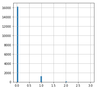
acc_labels.describe()
acc_labels.hist(bins=50, figsize=(5,5))
plt.show()
1
acc['accident type'].value_counts()
1
2
3
NONE    16219
A1       1313
Name: accident type, dtype: int64
1
acc['Time'].head()
1
2
3
4
5
6
0    1/1/2011 0:00
1    1/1/2011 2:00
2    1/1/2011 4:00
3    1/1/2011 6:00
4    1/1/2011 8:00
Name: Time, dtype: object
1
2
3
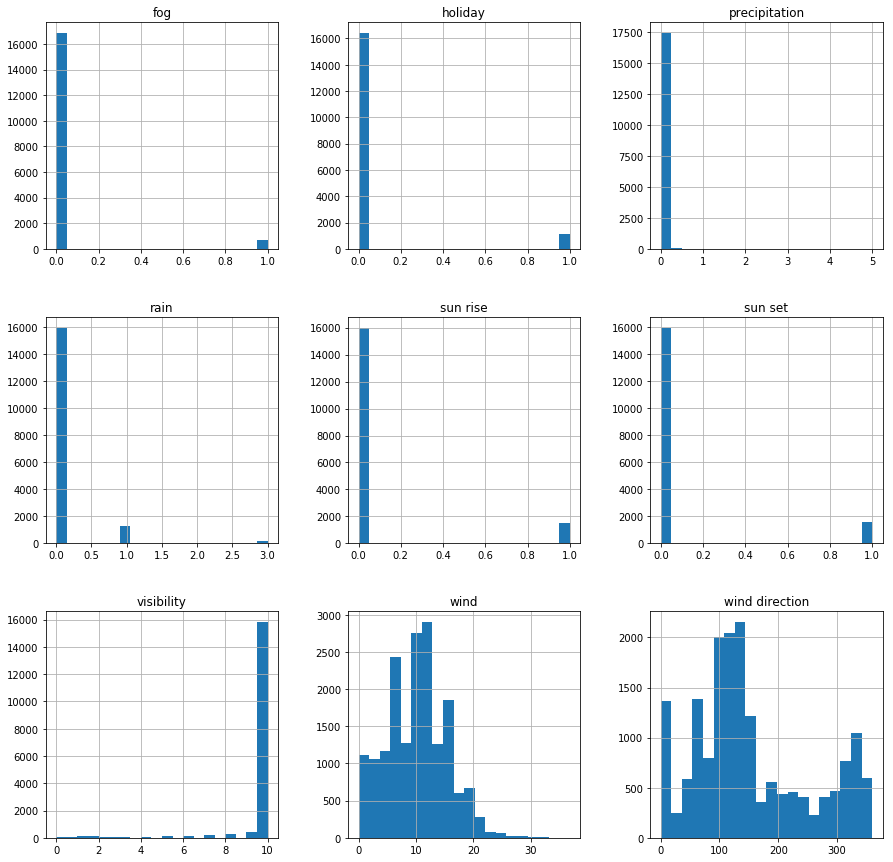
#各属性值的分布 ['holiday', 'precipitation', 'visibility', 'wind', 'wind direction', 'fog', 'rain', 'sun rise', 'sun set']
acc.hist(bins=20, figsize=(15,15))
plt.show()
1
2
3
4
5
#['Time', 'accident type', 'holiday', 'precipitation', 'visibility', 'wind', 'wind direction', 'fog', 'rain', 'sun rise', 'sun set'
from pandas.plotting import scatter_matrix

scatter_attributes = [ 'accident num','precipitation', 'visibility', 'wind', 'wind direction', 'fog', 'rain']
scatter_matrix(acc_all[scatter_attributes], alpha=0.2, figsize=(16, 16), diagonal='kde')
…
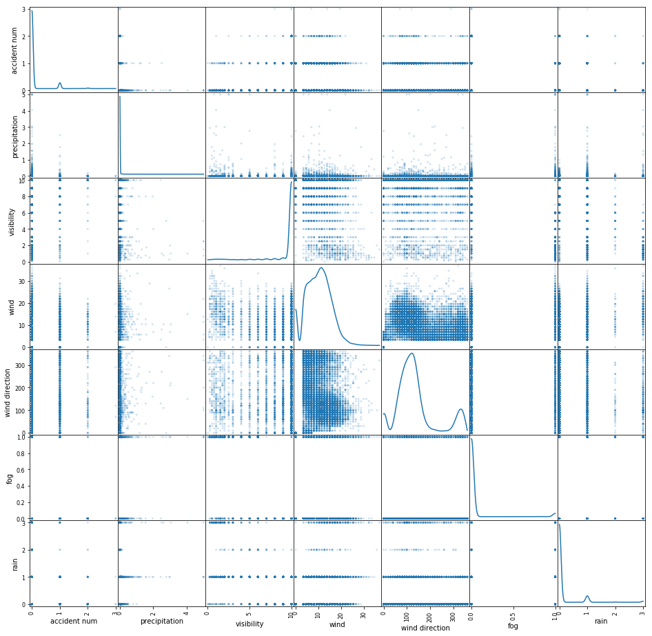
暂时只能看出wind和wind direction有较强关联性,各个属性同accident_num没有明显强关联性。计算一下各个属性的相关性系数看看
1
2
3
4
corr_attributes = ['accident num', 'precipitation', 'visibility', 'wind', 'wind direction', 'fog', 'rain','sun rise', 'sun set']
acc_corr = acc_all[corr_attributes]
corr_matrix = acc_all.corr()
corr_matrix['accident num'].sort_values(ascending=False)
各属性列同label列的关联系数
1
2
3
4
5
6
7
8
9
10
11
accident num      1.000000
wind              0.043940
rain              0.014107
fog               0.006532
precipitation     0.003703
sun set           0.001778
wind direction   -0.000414
visibility       -0.009250
holiday          -0.012781
sun rise         -0.023082
Name: accident num, dtype: float64
总体看起来风、雨、雾相关系数最大。风向、日出日落、假期、可视度(常理可视度影响应该会比较大)系数没有明显关联。
预处理
缺失值补齐
从’acc.info()’结果看来数据没有缺失
属性合并
暂无
分类值转数值
Time, accident type两个属性需要处理
1
acc.head()
| Time | accident type | holiday | precipitation | visibility | wind | wind direction | fog | rain | sun rise | sun set | |
|---|---|---|---|---|---|---|---|---|---|---|---|
| 0 | 1/1/2011 0:00 | A1 | 1 | 0.0 | 10.0 | 16.11 | 130 | 0 | 0 | 0 | 0 |
| 1 | 1/1/2011 2:00 | NONE | 1 | 0.0 | 10.0 | 10.36 | 130 | 0 | 0 | 0 | 0 |
| 2 | 1/1/2011 4:00 | NONE | 1 | 0.0 | 10.0 | 13.80 | 130 | 0 | 0 | 0 | 0 |
| 3 | 1/1/2011 6:00 | NONE | 1 | 0.0 | 10.0 | 16.11 | 130 | 0 | 0 | 1 | 0 |
| 4 | 1/1/2011 8:00 | NONE | 1 | 0.0 | 10.0 | 16.11 | 140 | 0 | 0 | 0 | 0 |
1
2
print(acc['Time'].head())
print(acc['Time'].tail())
检查时间转换的效果
1
2
3
4
5
6
7
8
9
10
11
12
0    1/1/2011 0:00
1    1/1/2011 2:00
2    1/1/2011 4:00
3    1/1/2011 6:00
4    1/1/2011 8:00
Name: Time, dtype: object
17527    14:00 31/12/2014
17528    16:00 31/12/2014
17529    18:00 31/12/2014
17530    20:00 31/12/2014
17531    22:00 31/12/2014
Name: Time, dtype: object
通过管道预处理数据
1
2
3
4
5
6
7
8
9
10
11
12
13
14
15
16
17
18
19
20
21
22
23
24
25
26
27
28
29
30
31
32
33
34
35
36
37
38
39
40
41
42
from sklearn.pipeline import Pipeline
from sklearn.preprocessing import StandardScaler
from sklearn.preprocessing import LabelBinarizer
from sklearn.pipeline import FeatureUnion
from sklearn.base import BaseEstimator, TransformerMixin
from datetime import datetime, date, time

class DataFrameSelector(BaseEstimator, TransformerMixin):
    def __init__(self, attribute_names):
        self.attribute_names = attribute_names
    def fit(self, x, y=None):
        return self
    def transform(self, x):
        return x[self.attribute_names].values

class LabelBinarizerPipelineFriendly(LabelBinarizer):
    def fit(self, X, y=None):
        """this would allow us to fit the model based on the X input."""
        super(LabelBinarizerPipelineFriendly, self).fit(X)
    def transform(self, X, y=None):
        return super(LabelBinarizerPipelineFriendly, self).transform(X)
    def fit_transform(self, X, y=None):
        print("debug:fit_transform len(x)=%d"%(len(X)))
        return super(LabelBinarizerPipelineFriendly, self).fit(X).transform(X)

class TimeAttribsTransformer(BaseEstimator, TransformerMixin):
    def __init__(self,time_from='01/01/2011 00:00'):
        self.from_dt = datetime.strptime(time_from, "%d/%m/%Y %H:%M")
    def fit(self,x, y=None):
        return self
    def __do_transform__(self, timeStr):
        #return timeStr
        day_time_splits = timeStr.split(' ')
        dt_format = "%d/%m/%Y %H:%M" if len(day_time_splits[0]) > len(day_time_splits[1]) else "%H:%M %d/%m/%Y"
        dt = datetime.strptime(timeStr, dt_format)
        dt_delta = dt-self.from_dt
        hours = dt_delta.days*24+dt_delta.seconds/3600
        return hours
    def transform(self,x,y=None):
        # hours from 2000/1/1 0:00
        time_sequence = np.array([self.__do_transform__(str(val[0])) for val in x])
        return np.c_[time_sequence]
1
2
3
4
5
6
7
8
9
10
11
12
13
14
15
16
17
18
19
20
21
22
23
24
25
26
27
28
29
30
31
32
from sklearn.pipeline import Pipeline

# 时间类数据处理
time_pipeline = Pipeline([
    # 数据选择
    ('selector', DataFrameSelector(time_attributes)),
     # 数据选择
    ('time_transformer', TimeAttribsTransformer())
])

# 分类型数据处理num_attributes
cat_pipeline = Pipeline([
    # 数据选择
    ('selector', DataFrameSelector(cat_attributes)),
    # 分类值独热编码
    ('label_binarizer', LabelBinarizerPipelineFriendly())
])

num_pipeline = Pipeline([
    # 数据选择
    ('selector', DataFrameSelector(num_attributes)),
    # 标准化:标准差标准化
    ('scaler', StandardScaler())
])

# pipeline集合
full_pipelines = FeatureUnion([
    ('num_pipeline',num_pipeline),
    ('cat_pipeline',cat_pipeline),
    ('time_pipeline',time_pipeline)
])
1
2
time_prepared = time_pipeline.fit_transform(acc[0:16])
print(time_prepared)
再次检查时间列的处理效果
1
2
3
4
5
6
7
8
9
10
11
12
13
14
15
16
[[ 0.]
 [ 2.]
 [ 4.]
 [ 6.]
 [ 8.]
 [10.]
 [12.]
 [14.]
 [16.]
 [18.]
 [20.]
 [22.]
 [24.]
 [26.]
 [28.]
 [30.]]
1
acc_prepared = full_pipelines.fit_transform(acc)
1
debug:fit_transform len(x)=17532
1
acc_prepared.shape
1
(17532, 11)
1
acc_prepared[10:14]
检查预处理后的数据
1
2
3
4
5
6
7
8
9
10
11
12
array([[ 3.81346997, -0.06465394,  0.2651457 ,  0.49370108, -0.21958904,
        -0.20362638, -0.27402253, -0.30910287, -0.31427953,  1.        ,
        20.        ],
       [ 3.81346997, -0.06465394,  0.2651457 ,  0.49370108, -0.21958904,
        -0.20362638, -0.27402253, -0.30910287, -0.31427953,  1.        ,
        22.        ],
       [-0.26222837, -0.06465394,  0.2651457 , -0.16112904, -0.32031364,
        -0.20362638, -0.27402253, -0.30910287, -0.31427953,  1.        ,
        24.        ],
       [-0.26222837, -0.06465394,  0.2651457 ,  0.05587862, -0.11886445,
        -0.20362638, -0.27402253, -0.30910287, -0.31427953,  1.        ,
        26.        ]])
用分类器分类看看
Linear Regression
先按照分类任务去做看看,将事故数据0,1,2,3次分别分作四类,建立分类器,看看分类出来的“预测”效果咋样。暂时先不做k-fold交叉验证只在测试集上看分类效果。
1
2
3
4
5
6
7
8
9
10
11
12
13
14
15
16
17
18
19
from sklearn.model_selection import cross_val_score
from sklearn.linear_model.stochastic_gradient import SGDClassifier

import warnings
import sklearn.exceptions
warnings.filterwarnings("ignore", category=sklearn.exceptions.UndefinedMetricWarning)

def cv_scores(model, dataset, labels):
    recall_score = cross_val_score(model, dataset, labels, scoring='recall_weighted',cv=8)
    print(recall_score)

    precision_score = cross_val_score(model, dataset, labels, scoring='precision_weighted',cv=8)
    print(precision_score)


clf_linear = SGDClassifier(max_iter=100)
#print(len(acc_prepared), len(acc_labels))
#clf_linear.fit(acc_prepared, acc_labels)
cv_scores(clf_linear, acc_prepared, acc_labels)
查看线性分类器的准确率和召回率
1
2
3
4
5
[0.92433911 0.92433911 0.9247606  0.92557078 0.92557078 0.92557078
 0.92557078 0.92557078]

[0.86751744 0.85440278 0.85518217 0.85668126 0.85668126 0.85668126
 0.85668126 0.        ]
Random Forest
1
2
3
4
5
from sklearn.ensemble import RandomForestClassifier

clf_rf = RandomForestClassifier(max_depth=4, random_state=0)
#clf_rf.fit(acc_prepared, acc_labels)
cv_scores(clf_rf, acc_prepared, acc_labels)
相比之下随机林的准确率和召回率看起来高多了
1
2
3
4
5
[0.92433911 0.92433911 0.9247606  0.92557078 0.92557078 0.92420091
 0.92557078 0.44383562]

[0.85440278 0.85440278 0.85518217 0.85668126 0.85668126 0.85658676
 0.85668126 0.82889293]
回归模型
用(T_min, T_max)去预测T_max+1时间的输出。
Linear Reggression
先写分数评估函数
1
2
3
4
5
6
7
8
9
10
11
12
13
14
15
from sklearn.metrics import precision_score
from sklearn.metrics import recall_score
from sklearn.metrics import f1_score
from sklearn.metrics import fbeta_score

def acc_predict(model, dataset, labels):
    label_values = labels.values
    predict = model.predict(dataset)
    predict_num = np.array([int(x) for x in predict])
    print( "precision:", precision_score(label_values, predict_num, average='weighted') )
    print( "recall:", recall_score(label_values, predict_num, average='weighted') )
    print( "f1:", f1_score(label_values, predict_num, average='weighted') )
    print( "fbeta 0.5:", fbeta_score(label_values, predict_num, beta=0.5, average='weighted') )
    print( "fbeta 1.0:", fbeta_score(label_values, predict_num, beta=1, average='weighted') )
    #在预测数据中存在实际类别没有的标签时报UndefinedMetricWarning
因为要使用(T_min, T_max)去预测T_max+1时间的输出所以需要队训练数据“掐头去尾”。
1
2
3
4
5
6
7
8
9
10
11
12
13
14
15
16
from sklearn.linear_model import LinearRegression

acc_prepared_rows = acc_prepared.shape[0]
acc_prepared = acc_prepared[:acc_prepared_rows-1,]
print(acc_prepared.shape)

acc_labels = acc_labels[1:]
print(acc_labels.shape)

data_len = acc_prepared.shape[0]
train_idx = int(data_len/2)
print(train_idx)
linear_reg = LinearRegression()
linear_reg.fit(acc_prepared[:train_idx,], acc_labels[:train_idx,])

acc_predict(linear_reg, acc_prepared[train_idx:,], acc_labels[train_idx:,])
回归分数看来结果不太理想,聊胜于无
1
2
3
4
5
6
7
8765
precision: 0.8076608288229538
recall: 0.8986995208761123
f1: 0.8507516012331187
fbeta 0.5: 0.8243624919032663
fbeta 1.0: 0.8507516012331187
mse: 0.13175906913073238
TODO
- 使用RNN做回归
- Grid Search / fine-tune Hyperparameter